rcicr implements reverse correlation image
classification, a psychophysics technique for visualizing
mental representations, for example of faces. It works in two
stages:
- Stimulus generation. A base image, such as a face photo, is combined with random visual noise. Each trial shows a pair: the “original” (base plus noise) and its “inverted” counterpart (base minus the same noise). On each trial the participant picks whichever of the two looks more like a target category, such as “trustworthy” or “happy”. This is a two-image forced-choice (2IFC) task.
- Classification image (CI). After data collection, the noise of every chosen original is added up and the noise of every chosen inverted image is subtracted. The average is the classification image: it shows which visual features drove the participant’s choices.
This vignette runs both stages on a tiny synthetic example. For the
full method, with several participants, scaling choices, z-maps and
informational value, see
vignette("reverse-correlation-walkthrough", package = "rcicr").
Example datasets and analysis scripts are in rcicr_examples.
1. Generate stimuli
generateStimuli2IFC() needs a square base image. To keep
this vignette self-contained we make a synthetic greyscale one. In a
real study you pass the path to your base face photo(s).
set.seed(42)
base_face_path <- tempfile(fileext = ".png")
png::writePNG(matrix(runif(64 * 64), 64, 64), base_face_path)
Now generate stimuli for a small task: 20 trials and one base image,
at a small size so the vignette builds quickly. A real study typically
uses img_size = 512 and several hundred trials (Dotsch
& Todorov, 2012).
stimulus_path <- tempfile("stimuli")

generateStimuli2IFC(
  base_face_files = list(face = base_face_path),
  n_trials        = 20,
  img_size        = 64,
  stimulus_path   = stimulus_path,
  seed            = 1,
  ncores          = 1,
  save_as_png     = FALSE # set to TRUE to also write stimulus PNGs to stimulus_path
)

rdata_file <- list.files(stimulus_path, pattern = "\\.Rdata$", full.names = TRUE)[1]
This writes an .Rdata file to stimulus_path
holding the noise parameters of every trial. That file is the
only link between stimulus generation and CI computation. Keep
it: every analysis function below needs it as its rdata
argument.
2. Collect (or, here, simulate) responses
In a real experiment you now run the 2IFC task and record, per trial,
which image each participant chose: 1 for the original,
-1 for the inverted one. This vignette has no participant,
so it simulates random responses. Random responses carry no signal, so
the resulting classification image shows nothing; never do this in a
real analysis.
3. Compute the classification image
generateCI() looks up the noise parameters of the
stimuli that were shown, weights them by the responses, and averages
them into one classification image.
ci <- generateCI(
  stimuli     = 1:20,
  responses   = responses,
  baseimage   = "face",
  rdata       = rdata_file,
  save_as_png = FALSE
)

names(ci)
#> [1] "ci"       "scaled"   "base"     "combined"
The result holds four pixel matrices:
-
ci$ciis the raw noise. -
ci$scaledis that noise rescaled for display. The default method,'independent', picks the lowest scaling constant that avoids clipping this particular image;?generateCIdescribes the others. -
ci$baseis the base image. -
ci$combinedoverlays the scaled noise on the base image.
image(ci$combined, col = gray.colors(256), axes = FALSE, asp = 1)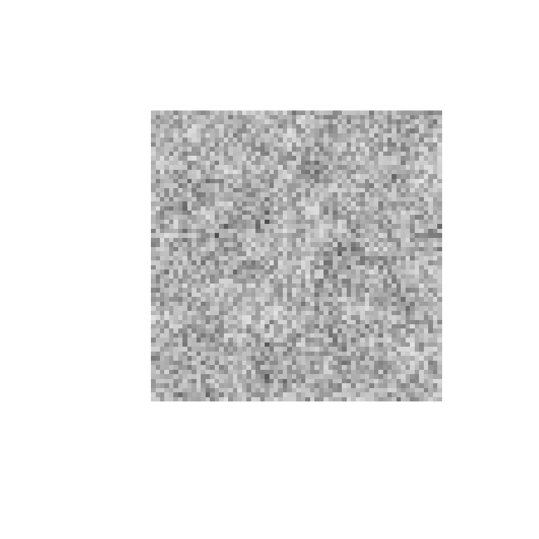
Because the responses were random, this classification image is just noise. With real data, patterns tied to the participants’ choices emerge here.
Next steps
-
batchGenerateCI()andbatchGenerateCI2IFC()compute one CI per participant or condition from a data frame. By default they put the whole batch on one scale withautoscale(), so the images can be compared by eye. -
computeInfoVal2IFC()computes the informational value: a z-score-like measure of how much signal a CI holds, compared with a simulated null distribution. -
plotZmap()shows which regions of a CI carry reliable signal.
Each function’s help page, such as ?generateCI or
?batchGenerateCI, lists its options and has runnable
examples.