A reverse correlation walkthrough
Source:vignettes/reverse-correlation-walkthrough.Rmd
reverse-correlation-walkthrough.RmdThis walkthrough covers a whole 2IFC reverse correlation study: designing it, generating stimuli, computing classification images for several participants, scaling them so they can be compared, and deciding whether what you see is signal or noise.
For the shortest working example, read
vignette("getting-started", package = "rcicr") instead.
Every code chunk here runs when the vignette is built, so an example that stops working with the current package fails the build instead of reaching you.
library(rcicr)

# CRAN asks that a vignette restore any graphical parameters it changes, so this
# records them and the last chunk puts them back. The show() helper below already
# restores the margins it sets, so this pair is a safety net -- and the pattern to
# copy into your own scripts.
old_par <- par(no.readonly = TRUE)
One small helper displays an image matrix throughout:
# zlim matters more than it looks. image() stretches whatever range it is given
# across the full palette, so without a fixed zlim every linear rescaling of the
# same image renders identically -- which would make the scaling comparison
# below silently meaningless. Pass zlim = c(0, 1) whenever the point is what the
# pixel values actually are; the default just stretches to the data's own range,
# which is what you want when only the structure matters.
show <- function(m, title, zlim = range(m, na.rm = TRUE)) {
  op <- par(mar = c(0, 0, 1.4, 0))
  # image() takes [x, y] with y increasing upwards, so a matrix indexed
  # [row, col] has to be transposed and flipped to display the right way up.
  image(t(m[nrow(m):1, ]), col = gray.colors(256), axes = FALSE, asp = 1, # nolint: seq_linter.
        main = title, zlim = zlim, useRaster = TRUE)
  par(op)
}
1. Installing
Install the current release from CRAN:
install.packages("rcicr")Use GitHub when you need to reproduce an analysis with a specific tagged release or test the unreleased development version:
# install.packages("remotes")
remotes::install_github("rdotsch/rcicr@v1.3.0") # a specific release
remotes::install_github("rdotsch/rcicr")         # the development version
remotes::install_github("rdotsch/rcicr@<commit-sha>") # pin an exact development snapshot
Record the version in your analysis script. For an unreleased GitHub install, also record the commit SHA and install that SHA when you return. A classification image is only reproducible with the exact code that computed it.
2. What the method does
On each trial a participant sees two images side by side. Both show the same base face: one with random visual noise added, the other with exactly the same noise subtracted. The participant picks whichever looks more like some category, for example more trustworthy, more masculine, or more like their own group.
Neither image contains a real signal. But suppose a participant reliably picks the image whose noise happens to resemble their mental picture of “trustworthy”. Averaging the noise of the images they chose, and subtracting the noise of the ones they rejected, then makes that picture visible. That average is the classification image.
3. Generating stimuli
generateStimuli2IFC() needs one or more
square base images. Here we draw a crude synthetic
face, so the vignette is self-contained and needs no image licence. In a
real study you pass the paths to your face photos.
n <- 64
rows <- matrix(seq(-1, 1, length.out = n), n, n)
cols <- matrix(seq(-1, 1, length.out = n), n, n, byrow = TRUE)
x <- cols
y <- -rows # row indices grow downwards, so flip to make +y point up

face <- exp(-(x^2 / 0.45 + y^2 / 0.75))                            # head
face <- face - 0.55 * exp(-(((x + 0.3)^2 + (y - 0.25)^2) / 0.012)) # left eye
face <- face - 0.55 * exp(-(((x - 0.3)^2 + (y - 0.25)^2) / 0.012)) # right eye
face <- face - 0.35 * exp(-(x^2 / 0.10 + (y + 0.42)^2 / 0.006))    # mouth
face <- (face - min(face)) / (max(face) - min(face))

base_face <- tempfile(fileext = ".png")
png::writePNG(face, base_face)

show(face, "synthetic base face", zlim = c(0, 1))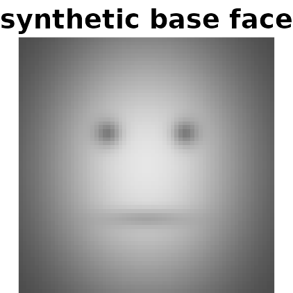
The base image must be square and already the size you
want. rcicr does not resize it, and stops with an
error if img_size disagrees.
stimulus_path <- tempfile("stimuli")
dir.create(stimulus_path)

generateStimuli2IFC(
  base_face_files = list(face = base_face),
  n_trials        = 120,
  img_size        = 64,
  stimulus_path   = stimulus_path,
  seed            = 1,
  nscales         = 3,
  ncores          = 1,
  save_as_png     = FALSE # TRUE in a real study: this writes the actual stimuli
)

rdata_file <- list.files(stimulus_path, pattern = "\\.Rdata$", full.names = TRUE)[1]
Real studies are much bigger than this. The defaults
(n_trials = 770, img_size = 512,
nscales = 5) follow published practice (Dotsch &
Todorov, 2012). Everything here is shrunk so the vignette builds in
seconds.
With save_as_png = TRUE you get two PNGs per trial per
base image, ..._ori.png and ..._inv.png. Those
are what participants see.
The .Rdata file is the important output
That file records the noise parameters behind every trial. It
is the only link between stimulus generation and analysis.
Nothing else records which noise pattern trial 57 actually showed.
Without it, the responses you collect can only be analysed after
regenerating the file from the seed and every generation setting, as
vignette("recipes", package = "rcicr") shows.
Back it up with your data. Every analysis function below takes it as
rdata.
4. Collecting responses
Run the task however you like (see “Running the task online” below). Per trial you need back:
- the stimulus number: which trial of the generated set was shown;
- the response:
1if the participant chose the original,-1if they chose the inverted one.
So that this walkthrough shows a real result rather than a grey smudge, we simulate three participants. All three have the same mental template and respond according to it, but with different amounts of inconsistency.
e <- new.env()
load(rdata_file, envir = e)
params <- e$stimuli_params[["face"]]

# The template is itself a noise image, so it is exactly expressible in the same
# basis the stimuli are drawn from.
set.seed(99)
template <- generateNoiseImage(rnorm(max(e$p$patchIdx)), e$p)

# Each trial's noise image, and how strongly it matches the template.
stack <- vapply(seq_len(nrow(params)),
                function(i) generateNoiseImage(params[i, ], e$p),
                matrix(0, 64, 64))
evidence <- apply(stack, 3, function(z) base::sum(z * template))
evidence <- evidence / sd(evidence)

# Three observers with the same template but increasing internal noise: the
# third is much less consistent than the first.
set.seed(7)
simulate <- function(internal_noise) {
  ifelse(evidence + rnorm(length(evidence), 0, internal_noise) > 0, 1, -1)
}

responses <- data.frame(
  participant = rep(c("p01", "p02", "p03"), each = nrow(params)),
  stimulus    = rep(seq_len(nrow(params)), 3),
  response    = c(simulate(0.5), simulate(1.5), simulate(3))
)

head(responses)
#>   participant stimulus response
#> 1         p01        1        1
#> 2         p01        2        1
#> 3         p01        3       -1
#> 4         p01        4       -1
#> 5         p01        5        1
#> 6         p01        6        1
Real data takes exactly this shape: one row per trial per participant.
5. Computing one classification image
ci_p01 <- generateCI(
  stimuli     = responses$stimulus[responses$participant == "p01"],
  responses   = responses$response[responses$participant == "p01"],
  baseimage   = "face",
  rdata       = rdata_file,
  save_as_png = FALSE
)

names(ci_p01)
#> [1] "ci"       "scaled"   "base"     "combined"
The returned list has four parts. Keep the first two apart:
-
ci: the raw classification image. This is the data; compute statistics from it. -
scaled:cirescaled into the 0–1 range a PNG can store. This is a display transformation: the method you pick changes how the image looks, not what it means. -
base: the base image. -
combined:scaledoverlaid onbase. This is what gets written to disk.
Did we recover the template the simulated observer was using?
show(template, "true template")
show(ci_p01$ci, "recovered CI")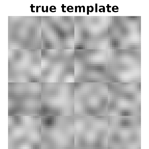
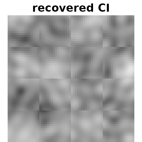
With real participants there is no template to compare against; finding it is the whole point of the technique. Section 8 shows how to tell signal from noise when you cannot peek at the answer.
generateCI2IFC() does the same with an older argument
list, kept so that analysis scripts written years ago still run. New
code should use generateCI().
6. Scaling
Scaling decides what the image looks like. generateCI()
offers four methods, and choosing one is a reporting decision, not a
cosmetic one.
for (method in c("none", "constant", "matched", "independent")) {
  res <- generateCI(
    stimuli     = responses$stimulus[responses$participant == "p01"],
    responses   = responses$response[responses$participant == "p01"],
    baseimage   = "face", rdata = rdata_file, save_as_png = FALSE,
    scaling     = method, scaling_constant = 0.5
  )
  # $scaled, not $combined, so the effect of scaling is visible rather than
  # hidden under the base image -- and zlim fixed to the displayable range, so
  # that what you see is the actual pixel values.
  show(res$scaled, method, zlim = c(0, 1))
}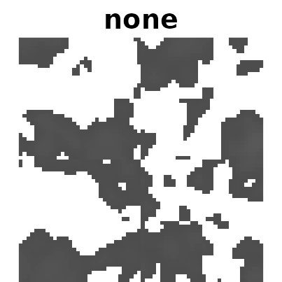

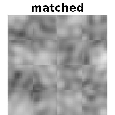
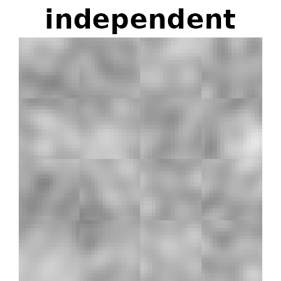
The four panels differ as follows.
none leaves the raw CI, whose values
straddle zero and span only about ±0.04. Nothing in that range can be
displayed: negative pixels fall outside 0–1 entirely (blank above), and
positive ones are so close to zero that they render near-black. A PNG
clips out-of-range values rather than dropping them, so written to disk
almost the whole image would be black. You always need some scaling.
constant with
scaling_constant = 0.5 gives a flat grey. The constant is
more than ten times the CI’s actual range, so every difference is
squeezed into a sliver of the palette. Choose a constant with the data’s
range in mind: too large destroys the signal just as surely as too small
clips it.
matched and
independent both use the available range.
They look similar here only because this base image already spans nearly
0–1; on a real photograph with a narrower range they diverge.
-
independent(the default) picks, for each image separately, the smallest constant that avoids clipping. Every CI uses its full range, so two CIs scaled this way cannot be compared with each other: each got a different constant. -
constantdivides by a fixed constant you choose, so several CIs stay on one scale. Use this, orautoscale(), when comparing conditions. -
matchedmatches the CI’s intensity range to the base image’s. This is nonlinear. -
nonedoes nothing; values outside 0–1 are clipped on save.
Whichever you choose, ci$ci is untouched, so statistics
computed from it do not depend on the display choice.
7. Several participants at once
batchGenerateCI() splits a data frame by a grouping
column and computes one CI per group.
cis <- batchGenerateCI(
  data        = responses,
  by          = "participant",
  stimuli     = "stimulus",
  responses   = "response",
  baseimage   = "face",
  rdata       = rdata_file,
  save_as_png = FALSE
)
names(cis)
#> [1] "face_participant_p01" "face_participant_p02" "face_participant_p03"
To compare conditions rather than participants, point by
at the condition column.
These CIs are already on one scale: by default,
batchGenerateCI() computes them unscaled and then calls
autoscale(), which finds one constant that fits all of them
without clipping any. For CIs you computed separately, call
autoscale() yourself. On this batch it gives the same
result:
scaled <- autoscale(cis, save_as_pngs = FALSE)
#> Using scaling factor constant:0.0384382346907274

for (nm in names(scaled)) {
  # $scaled, not $combined -- see the note below.
  show(scaled[[nm]]$scaled, sub(".*_", "", nm), zlim = c(0, 1))
}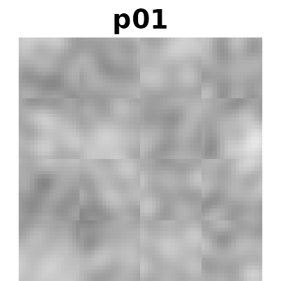
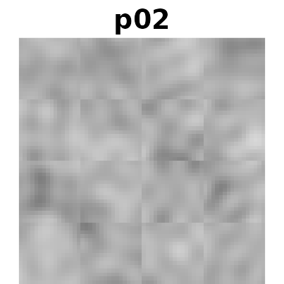
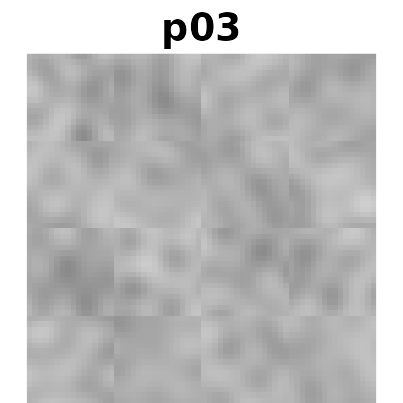
p01 should look cleanest and p03 weakest.
They share a template but differ in how consistently they applied it,
which is what internal noise means in practice.
After autoscale(), look at $scaled
autoscale() rewrites $scaled and
leaves $combined exactly as it was, on
purpose: an existing analysis script that plots $combined
keeps producing the same image.
This catches people out after batchGenerateCI(). That
function scales with 'none', so its $combined
overlays the unscaled noise and looks almost blank. To see the
autoscaled noise over the base image, build the overlay yourself:
p01 <- scaled[["face_participant_p01"]]
show((p01$scaled + p01$base) / 2, "p01 over base", zlim = c(0, 1))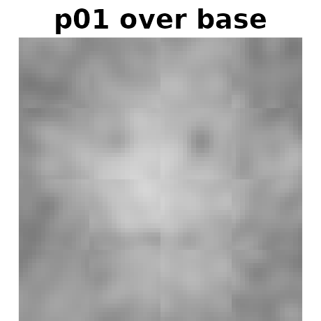
That expression is exactly what
autoscale(save_as_pngs = TRUE) writes to disk.
The argument is save_as_pngs. Older tutorials show
saveasjpegs, which no longer exists.
8. Is there actually signal?
Two tools answer different questions.
computeInfoVal2IFC() gives one number
per CI: a z-score for how much stronger this CI is than one built from
random responses. Values above about 1.96 indicate reliable signal.
It needs a reference distribution simulated under the same task parameters. That takes a long time to build, so the code is shown but not run here:
# Slow: simulates `iter` classification images from random responses. Do this once
# per stimulus set; the result is cached back into the .Rdata file.
generateReferenceDistribution2IFC(rdata_file, iter = 10000)

computeInfoVal2IFC(target_ci = ci_p01, rdata = rdata_file)plotZmap(), or
generateCI(zmap = TRUE), answers the spatial question:
which regions of the image carry reliable signal.
zmap_dir <- tempfile("zmaps")

ci_z <- generateCI(
  stimuli     = responses$stimulus[responses$participant == "p01"],
  responses   = responses$response[responses$participant == "p01"],
  baseimage   = "face", rdata = rdata_file, save_as_png = FALSE,
  zmap = TRUE, zmapmethod = "quick", threshold = 1.5,
  zmaptargetpath = zmap_dir, zmapdecoration = FALSE
)
# Pixels that did not clear the threshold are set to NA.
range(ci_z$zmap, na.rm = TRUE)
#> [1] -2.208394  3.442531
mean(!is.na(ci_z$zmap)) # fraction of the image flagged
#> [1] 0.1337891
Choose the threshold by looking at the range, not by
habit. zmapmethod = "quick" z-scores a blurred CI
across the pixels of that one image. Its values are relative to
the image’s own spatial structure, not z-scores against a null
distribution, and their spread shrinks as the image gets smaller or the
blur wider. Here the whole map spans roughly ±1.7, so the default
threshold = 3 would have returned a blank map. That is not
evidence of no signal; it is the wrong ruler.
zmapmethod = "t.test" is the inferential counterpart: a
per-pixel t-test across trials. It is slower, but its statistic means
what it looks like. Neither method corrects for multiple comparisons
across pixels, so treat both as exploratory.
9. Running the task online
rcicr generates stimuli and analyses responses; it does
not run experiments. The stimulus PNGs are ordinary image files, so any
platform that can show two images and record a choice will do:
Qualtrics, jsPsych, Gorilla, PsychoPy, or a page of your own.
Get two things right:
-
Record the stimulus number, not the filename you
happened to serve. The number is what indexes into the
.Rdatafile. -
Record which of the pair was chosen as
1(original) or-1(inverted), and be certain which is which. A systematic flip inverts every classification image you compute, and the result looks like a plausible mental representation of the opposite trait.
Worked examples and analysis scripts: https://github.com/rdotsch/rcicr_examples/
10. Citing
citation("rcicr")citation("rcicr") cites the software. If you use the
technique, also cite the method: Dotsch and Todorov (2012) doi:10.1177/1948550611430272, and for a practical primer
Brinkman, Todorov and Dotsch (2017) doi:10.1080/10463283.2017.1381469.