Short answers to questions that come up once the basics in
vignette("reverse-correlation-walkthrough", package = "rcicr")
are in place. Each recipe runs at a small size so this vignette builds
in seconds; real studies use img_size = 512 and several
hundred trials.
A stimulus set and a simulated participant
The recipes share one stimulus set: a synthetic face (no photo, so no image licence) and 120 trials.
n <- 64
x <- matrix(seq(-1, 1, length.out = n), n, n, byrow = TRUE)
y <- -matrix(seq(-1, 1, length.out = n), n, n)
face <- exp(-(x^2 / 0.45 + y^2 / 0.75))
face <- face - 0.55 * exp(-(((x + 0.3)^2 + (y - 0.25)^2) / 0.012))
face <- face - 0.55 * exp(-(((x - 0.3)^2 + (y - 0.25)^2) / 0.012))
face <- face - 0.35 * exp(-(x^2 / 0.10 + (y + 0.42)^2 / 0.006))
face <- (face - min(face)) / (max(face) - min(face))
base_face <- tempfile(fileext = ".png")
png::writePNG(face, base_face)

stimulus_path <- tempfile("stimuli")
generateStimuli2IFC(list(face = base_face), n_trials = 120, img_size = n,
                    stimulus_path = stimulus_path, seed = 1, nscales = 3,
                    ncores = 1, save_as_png = FALSE)
rdata_file <- list.files(stimulus_path, pattern = "\\.Rdata$", full.names = TRUE)[1]
So that the results show something, a simulated participant responds
according to a hidden template. evidence is how strongly
each trial’s noise matches it.
e <- new.env()
load(rdata_file, envir = e)
set.seed(99)
template <- generateNoiseImage(rnorm(max(e$p$patchIdx)), e$p)
evidence <- vapply(seq_len(120), function(i) {
  base::sum(generateNoiseImage(e$stimuli_params$face[i, ], e$p) * template)
}, numeric(1))
evidence <- evidence / sd(evidence)
set.seed(7)
choice <- ifelse(evidence + rnorm(120) > 0, 1, -1) # 1: original chosen, -1: inverted
Noise-only stimuli
To show noise without a face (for a task about textures, say, or to
inspect the noise itself), use a uniform mid-grey base image. A uniform
image has no contrast to maximize, so pass
maximize_baseimage_contrast = FALSE.
grey <- tempfile(fileext = ".png")
png::writePNG(matrix(0.5, n, n), grey)
noise_path <- tempfile("noise")
generateStimuli2IFC(list(grey = grey), n_trials = 4, img_size = n,
                    stimulus_path = noise_path, seed = 1, nscales = 3, ncores = 1,
                    maximize_baseimage_contrast = FALSE)
ori <- png::readPNG(file.path(noise_path, "rcic_grey_1_00001_ori.png"))
inv <- png::readPNG(file.path(noise_path, "rcic_grey_1_00001_inv.png"))
show(ori, "trial 1, original", zlim = c(0, 1))
show(inv, "trial 1, inverted", zlim = c(0, 1))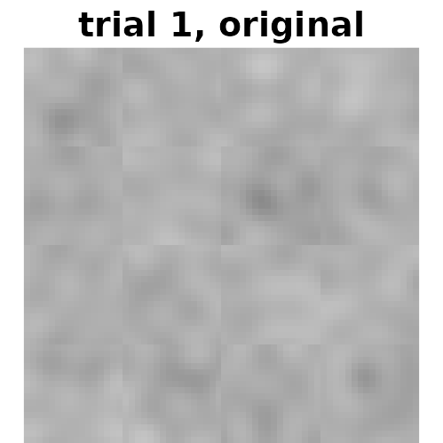
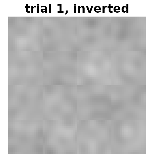
These are ordinary 2IFC stimuli: the stimulus PNGs average the noise
with the base, so on a grey base the noise appears at half contrast, and
the .Rdata file is analysed as usual. For the noise at full
contrast, for display rather than for a task, ask for it back as a data
frame, one column per trial:
noise <- generateStimuli2IFC(list(grey = grey), n_trials = 4, img_size = n, seed = 1,
                             nscales = 3, ncores = 1, return_as_dataframe = TRUE,
                             maximize_baseimage_contrast = FALSE,
                             save_as_png = FALSE, save_rdata = FALSE)
# The same scaling the stimuli use, without the base: most noise falls in [-0.3, 0.3].
noise_1 <- pmin(pmax((matrix(noise[[1]], n, n) + 0.3) / 0.6, 0), 1)
show(noise_1, "trial 1 noise, full contrast", zlim = c(0, 1))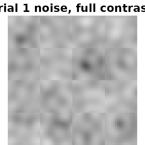
Ratings instead of a two-image choice
generateCI() weights each trial’s noise by its response,
so any numeric response works, not only 1/-1.
If participants rated each stimulus on a scale, recode the scale so that
its midpoint is 0 and its direction is the one you want the
classification image to show. Here a 1–4 scale (“not at all” to “very
much”) is recoded to -2, -1, 1, 2:
set.seed(11)
rating <- as.integer(cut(evidence + rnorm(120, 0, 0.7), c(-Inf, -0.7, 0, 0.7, Inf)))
table(rating)
#> rating
#>  1  2  3  4
#> 34 30 26 30

ci_rating <- generateCI(1:120, c(-2, -1, 1, 2)[rating], "face", rdata_file,
                        save_as_png = FALSE)
cor(as.vector(ci_rating$ci), as.vector(template))
#> [1] 0.5764985
Check the direction. Recoded the wrong way round, the scale gives the anti-classification image, and that looks like a plausible face too. With real data there is no template to compare against: compare instead with a CI whose direction you know, such as a 2IFC CI for the same target, or check that the expected features appear.
Responses must be numeric and complete. A missing rating, a factor,
or TRUE/FALSE stops generateCI()
with an error naming the trials, rather than returning an image of
NAs. Drop unanswered trials from stimuli and
responses alike.
Matching the InfoVal reference to the design
computeInfoVal2IFC() compares a classification image
with a reference distribution: CIs built from random responses. The
reference must match the CI’s design. When it does not, the InfoVal is
miscalibrated.
When some trials were dropped
Say 20 trials were dropped because the participant did not respond in time. The CI is built from 100 stimuli; the default reference uses all 120.
kept <- setdiff(1:120, seq(3, 120, by = 6))
ci_kept <- generateCI(kept, choice[kept], "face", rdata_file, save_as_png = FALSE)
attr(ci_kept, "trial_design")$stimuli[1:10]
#>  [1]  1  2  4  5  6  7  8 10 11 12
generateCI() records the stimuli it used, so the
matching reference is one argument away. The default call says the two
differ:
default <- computeInfoVal2IFC(ci_kept, rdata_file, iter = 10000)
#> This classification image was built from 100 of the 120 saved stimuli, but the reference is built over 120. Brinkman et al. (2019) require the reference to use the stimuli the CI was built from. To score it that way, pass reference_stimuli = attr(<your CI>, "trial_design")$stimuli.
#> InfoVal reference computed with reference_method = "gram". References from rcicr 1.5.0 and earlier used "images"; pass reference_method = "images" to reproduce them bit for bit.
matched <- computeInfoVal2IFC(ci_kept, rdata_file, iter = 10000,
                              reference_stimuli = attr(ci_kept, "trial_design")$stimuli)
#> InfoVal reference computed with reference_method = "gram". References from rcicr 1.5.0 and earlier used "images"; pass reference_method = "images" to reproduce them bit for bit.
c(default = default, matched = matched)
#>  default  matched
#> 3.837017 2.423099
Fewer stimuli give a noisier CI, so its norm is larger under random
responding too: against the full-set reference, the default InfoVal is
inflated. Each reference is simulated once and stored in the
.Rdata file for later calls.
A masked classification image
A CI computed with a mask holds NA in the
masked pixels. Its InfoVal is computed over the unmasked pixels, against
a reference over the same pixels. Here only the eye region is kept (in a
mask, 0 is masked):
mask <- matrix(0, n, n)
mask[18:30, 10:54] <- 1
ci_eyes <- generateCI(1:120, choice, "face", rdata_file, mask = mask, save_as_png = FALSE)
infoval_eyes <- computeInfoVal2IFC(ci_eyes, rdata_file, iter = 10000)
#> InfoVal reference computed with reference_method = "gram". References from rcicr 1.5.0 and earlier used "images"; pass reference_method = "images" to reproduce them bit for bit.
show(ci_eyes$ci, "CI, eye region only")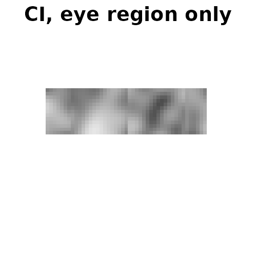
infoval_eyes
#> [1] 1.384019
An InfoVal over part of the image is not comparable with one over the whole image.
Several classification images at once
batchComputeInfoVal2IFC() scores a list of CIs, such as
the result of batchGenerateCI2IFC(), and simulates each
distinct reference once:
set.seed(3)
data <- data.frame(
  participant = rep(c("p1", "p2", "p3"), each = 120),
  stimulus    = rep(1:120, 3),
  response    = c(ifelse(evidence + rnorm(120, 0, 0.5) > 0, 1, -1),
                  ifelse(evidence + rnorm(120, 0, 2) > 0, 1, -1),
                  sample(c(1, -1), 120, replace = TRUE))
)
cis <- batchGenerateCI2IFC(data, "participant", "stimulus", "response", "face",
                           rdata_file, save_as_png = FALSE)
infovals <- batchComputeInfoVal2IFC(cis, rdata_file, iter = 10000)
round(infovals, 2)
#> face_participant_p1 face_participant_p2 face_participant_p3
#>                6.32                0.73                0.20
The third participant answered at random, and scores near 0.
A CI averaged over participants
No reference is defined for a CI that averages several participants
(or repeated presentations of the same stimulus): every reference
assumes one response per stimulus from one responder.
computeInfoVal2IFC() returns a number but says it is not
calibrated.
ci_group <- generateCI(data$stimulus, data$response, "face", rdata_file,
                       participants = data$participant, save_as_png = FALSE, n_cores = 1)
infoval_group <- computeInfoVal2IFC(ci_group, rdata_file, iter = 10000)
#> This classification image averages 3 participants. Every InfoVal reference in rcicr assumes one response per stimulus from one responder, and none is defined for this design, so this InfoVal is not calibrated for it. Where each participant saw every stimulus once, compute InfoVal for each participant's own CI instead.
infoval_group
#> [1] -3.524378
Averaging shrinks the CI’s norm, so against a single-responder reference the group CI scores below zero, although one of its participants scored 6.3 on their own. Score each participant’s own CI instead, as above.
Reproducing a number from an earlier version
A classification image or InfoVal reported years ago can be reproduced in two ways.
Run the version that computed it
This reproduces everything the file already stores exactly. A
reference the old release has to simulate anew also needs the original
session’s RNGkind(), which files from before
rng_kind was stored do not record, and the same BLAS
library. For a release, use the version your analysis script or its
session info records. A development install from GitHub is identified
only by its commit SHA, since snapshots share a version number: install
the SHA you recorded,
remotes::install_github("rdotsch/rcicr@<commit-sha>"),
or keep the library it was installed in.
p$generator_version in the .Rdata file (in
files from 0.3.3 on) names the version that generated the
stimuli, which need not be the one that analysed them. Install that
release into a library of its own, so your current installation stays as
it is, and load it in a fresh R session:
dir.create("rcicr-1.4.1")
remotes::install_github("rdotsch/rcicr@v1.4.1", lib = "rcicr-1.4.1")
library(rcicr, lib.loc = "rcicr-1.4.1")
Older releases import packages this one no longer needs;
install_github() installs those too.
Recompute with the current version
Classification images come out the same unless NEWS.md
lists your situation under “Reproducibility impact”, in the releases
after the one you used. For a version before 1.1.0, check
ChangeLog too: NEWS.md starts at 1.1.0.
Their file names can differ, though, for per-participant images from
a GitHub install before 1.3.0. In affected versions, a direct
generateCI() call with participants and
save_individual_cis = TRUE could save an image under
another participant’s name. Rerunning such a version reproduces the
wrong names; recomputing with this one gives the right names, so
comparing old and new files by name can turn up differences where there
are none. The individual-CI
filename advisory explains how to tell whether you are affected.
CRAN releases never carried the bug.
An InfoVal depends on the reference distribution stored in the
.Rdata file:
-
A reference stored by 1.4.0 or later is reused as
stored, so its InfoVal does not change, as long as no older
rcicr has since replaced its norms. Such a reference carries a
sourcemarker;vignette("stored-data", package = "rcicr")shows where it sits for each way a reference is stored. -
A reference drawn with a
response_seedis kept as stored, whichever method you ask for. -
Any other reference is rebuilt the first time, with
a message that the new InfoVal supersedes earlier ones. By default it is
computed through the stimulus Gram matrix, which differs from the
calculation of 1.5.0 and earlier only by rounding;
reference_method = "images"is that earlier calculation, unchanged. A file generated withseed = NULLcannot rebuild its reference; the error names the call that stores a reproducible one instead.
To rebuild a reference the way earlier versions did, store it with
generateReferenceDistribution2IFC() and
reference_method = "images", passing the original
iter (the length of the stored norms, if the file still
holds them), the original response_seed if there was one,
and, when the base images have parameters of their own, the
classification image’s baseimage. Later
computeInfoVal2IFC() calls reuse it. Whether it then
matches the old reference exactly depends on what changed after your
version, so read the “Reproducibility impact” entries in
NEWS.md for every later release (and
ChangeLog, for versions before 1.1.0). It also needs the
original session’s random number generator and BLAS library;
sessionInfo() names the BLAS, and lists the generator only
when it differs from R’s default.
Here both methods score the same classification image, each on its own copy of the file:
ci_all <- generateCI(1:120, choice, "face", rdata_file, save_as_png = FALSE)

gram_file <- tempfile(fileext = ".Rdata")
file.copy(rdata_file, gram_file)
generateReferenceDistribution2IFC(gram_file, iter = 1000, ncores = 1)
#> InfoVal reference computed with reference_method = "gram". References from rcicr 1.5.0 and earlier used "images"; pass reference_method = "images" to reproduce them bit for bit.
infoval_gram <- computeInfoVal2IFC(ci_all, gram_file, iter = 1000)

images_file <- tempfile(fileext = ".Rdata")
file.copy(rdata_file, images_file)
generateReferenceDistribution2IFC(images_file, iter = 1000, ncores = 1,
                                  reference_method = "images")
infoval_images <- computeInfoVal2IFC(ci_all, images_file, iter = 1000)
c(gram = infoval_gram, images = infoval_images, difference = infoval_images - infoval_gram)
#>         gram       images   difference
#> 2.725105e+00 2.725105e+00 1.065814e-14
Real references use iter = 10000; the smaller one here
keeps the slower "images" calculation quick.
When the .Rdata file is lost
The .Rdata file can be regenerated:
generateStimuli2IFC() draws the same stimuli again from the
same seed and settings. The release gate checks, on every release, that
this version draws the same stimulus parameters as 1.0.1, bit for bit,
in the configurations it runs; files from earlier versions are not
compared. Two kinds of stimulus set cannot be regenerated at all: those
generated with seed = NULL, which seeds from the clock and
stores no seed, and those generated before 0.3.0, which drew 4096
parameters per trial where later versions draw 4092, so every trial
after the first comes out different. Both can still be analysed from a
surviving .Rdata file. Regenerating any other set
needs:
-
The seed. It is in the name of the
.Rdatafile,<label>_seed_<seed>_time_<timestamp>.Rdata, and of every stimulus PNG,<label>_<base label>_<seed>_<trial>_ori.png. -
Every generation setting:
n_trials,img_size,nscales,noise_type,sigma(for Gabor noise) anduse_same_parameters. The defaults have been the same since 1.0.1: 770 trials, 512 pixels, 5 scales, sinusoid noise,sigma = 25, shared parameters. -
The base labels, the names in
base_face_files. They are the keysgenerateCI(baseimage = )looks up, so analysis code written for the original file needs them. When each base image had parameters of its own, their order matters too, because each base’s parameters are drawn in turn. -
The same random number generator. Stimuli are drawn
with
runif(), so this matters only if the original session changed R’s default generator.
ncores, label and
maximize_baseimage_contrast do not change the parameters.
Some values earlier versions accepted now stop with an error; use the
value the old version actually applied. An unrecognised
noise_type such as "Gabor" produced sinusoid
noise, and a fractional n_trials its whole part, which the
number of PNGs confirms. NEWS.md lists the input checks
added in each release.
The base images are not needed for the classification image’s noise
(ci) or its InfoVal: those depend only on the stimulus
parameters and the noise basis, so a uniform grey stand-in gives the
same values as the original images would. A uniform image needs
maximize_baseimage_contrast = FALSE. Everything that
involves the base does need it: base,
combined, and scaled under
scaling = "matched", which maps the CI onto the base
image’s range.
Checking the settings against the stimulus PNGs
If you still have the stimulus PNGs, they confirm the settings. The
number of _ori files per base image gives
n_trials, and their size img_size.
checkStimulusPNGs2IFC() checks the rest, trial by trial and
without the base images: an original and an inverted stimulus hold the
same base, so their difference is the trial’s noise alone.
Here an archive keeps only its PNGs:
archive <- tempfile("archive")
generateStimuli2IFC(list(face = base_face), n_trials = 10, img_size = n,
                    stimulus_path = archive, seed = 5, nscales = 3, ncores = 1)
unlink(list.files(archive, pattern = "\\.Rdata$", full.names = TRUE))
head(list.files(archive), 2)
#> [1] "rcic_face_5_00001_inv.png" "rcic_face_5_00001_ori.png"
regenerate() writes a stimulus file for candidate
settings, over a grey stand-in. checkStimulusPNGs2IFC()
then gives, per trial, the share of unclipped pixels that agree with
that file’s noise. It needs the archive’s label and
seed, because the PNG names carry them:
regenerate <- function(nscales) {
  grey <- tempfile(fileext = ".png")
  png::writePNG(matrix(0.5, n, n), grey)
  path <- tempfile("regenerated")
  generateStimuli2IFC(list(face = grey), n_trials = 10, img_size = n, stimulus_path = path,
                      seed = 5, nscales = nscales, ncores = 1, save_as_png = FALSE,
                      maximize_baseimage_contrast = FALSE)
  list.files(path, pattern = "\\.Rdata$", full.names = TRUE)
}
lowest_share <- function(rdata) {
  min(checkStimulusPNGs2IFC(rdata, archive, label = "rcic", seed = 5)$share)
}
setNames(vapply(files, lowest_share, numeric(1)), paste("nscales =", candidates))
#> nscales = 3 nscales = 5
#>  1.00000000  0.02050781
The right settings match every trial. With several base images, look
at every base label in the result: the first base’s parameters are drawn
the same way whether or not use_same_parameters is right,
so only the later bases show a wrong value. In the configurations measured,
a wrong nscales, seed, noise type, base order or
use_same_parameters agreed on 2.1% to 7.4% of pixels per
trial. A Gabor sigma of 24 where the PNGs used 25, though,
agreed on 95% to 99.6%. So compare candidates on the same PNGs, and keep
the one that scores highest. PNGs written by 1.5.0 and earlier show a
few pixels above white as dark, which lowers even the right candidate’s
share, to 0.986 in the lowest trial measured.
With the right settings found, regenerate the file once more with the
original base images and maximize_baseimage_contrast, and
use it as the .Rdata file. Its ci is the one
this version computes from the original file. Compared with a
ci an earlier version computed, the differences listed
under “Reproducibility impact” in NEWS.md apply, as in the
recipe above; some are rounding of about one unit in the last place. The
InfoVal reference stored in the lost file is gone, though: a regenerated
file holds none, so the first computeInfoVal2IFC()
simulates one with the current defaults. To rebuild the reference the
original analysis used, pass its settings as in “Reproducing a number
from an earlier version” above; if those settings are unknown, the
original InfoVal cannot be recovered exactly. Its stored base matches
only if this version reads the images as the original one did;
NEWS.md lists where that changed, such as base images with
an alpha channel before 1.4.0. Where it did, regenerate the display data
with the original version instead.